Classical Least Squares for Vapor Phase Quantitative Analysis
Contents
Introduction
Classical Least Squares (CLS) is a multivariate data reduction technique used for quantitative analysis of infrared spectra.
CLS is often used for the analysis of complex mixtures of gases (vapor phase samples), for instance combustion processes. CLS requires spectra of pure compounds of known concentrations, known as a 'standard' or 'calibration' spectrum. In some cases you may need only one standard for a given compound, if the concentration vs. absorbance curve is linear. Often, however, the absorbance will fall off at higher concentrations, so the calibration curve is not linear. In this case, for a more accurate measurement, it is necessary to provide more calibration spectra at a range of concentrations.
Peak Spectroscopy Software's CLS implementation is based on the 'multi-band weighting' technique combined with standard-bracketed interpolation, providing robust and sensitive concentration measurements.
The latest release of Peaks can be downloaded here.
A pdf version of this manual is available here: Peak_CLS.pdf
The sample method referred to in this document can be downloaded from c3f8_cls_method.zip
CLS is installed with Peaks. Although included in the Peaks installation and trial version, CLS is an add-on package requiring an additional license. Please contact peaks@tds.net to get a CLS license.
This manual is not meant to explain the CLS mathematics. There are many fine sources for this information, please see the References section.
Overview
A CLS method consists of analytes, which are the compounds that need to be quantified. An analyte needs at least one 'standard'. A standard is a spectrum of the pure analyte acquired at known concentration, temperature, pathlength and pressure. Standards require Analytical Regions to be defined, which are spectral regions in which the analyte has characteristic absorbances. In addition, Interferents can be assigned to a Standard. An Interferent is the spectrum of a pure compound which also has absorbance in the Analytical Regions assigned to the Standard, and which may be present in samples measured in the field. In practice, the Interferents are often other Analytes in the method.
A CLS method can be seen as a hierarchy. A method consists of Analytes. An Analyte consists of Standards. A Standard consists of 1) Analytical Region(s) and 2) possible Interferents. An Interferent is a spectrum which may also have absorbances in the Standard's Analytical Region(s), which would interfere with the calculation of the Standard's concentration if not taken into account.
The results of a CLS prediction follow the same Analyte/Standard/Region hierarchy. For a given sample and standard, a separate prediction is performed for each region defined for the standard. These individual region results are combined using a weighted average, a technique known as 'Multi-Band Weighting' (see reference 2). There is a MBW result for each standard for the analyte. The two standards whose MBW results most closely 'bracket' the predicted results are used to interpolate a final result for the analyte. So, there is a CLS prediction result for each region, a MBW result for each standard, and an interpolated result for each analyte.
If the sample cannot bracketed by the standards in the CLS method, the result is extrapolated from the nearest standard. Interpolated results are more accurate than extrapolated results. For this reason, the standards in the method should include concentrations that encompass the possible sample concentrations found in the field. Also, absorbance is not always linear with concentration. At higher concentrations, absorbance can fall off from a straight line. For this reason, it is again important to have enough standards with varying concentrations across the range of possible concentrations in the field.
The CLS Tool
The CLS tool is in the Peaks 'Quant & Identification' Toolbox. The CLS tool has these tabs:

Each of these tabs will now be explained.
The Method Tab
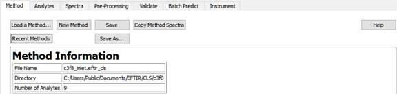
On this tab, methods are loaded, created, and saved.
 |
Load an existing method from disk |
 |
Shows a list of the last 10 methods that were loaded. |
 |
Create a new, blank, method |
 |
Save the current method. |
 |
Prompt for a filename for saving the current method. |
 |
Copy all of the method spectra to another folder. |
A sample method named c3f8_inlet is included with the installation in the folder 'C:\Users\Public\Documents\PeakSpectroscopy\CLS'.
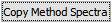
The Analytes Tab
An analyte is a compound of interest, the concentration of which you want to measure using a CLS method.
This screen shot assumes you have loaded the c3f8_inlet method. On this Analytes tab are two sub-tabs: Analytes and Computed Values. On the Analytes sub-tab, Analytes are created, edited and removed.
There is one row in the Analyte table for each analyte. The columns in the table are labeled 'Name', 'Status' and 'Units', Report Results', 'Bias Offset' and 'Bias Slope'.
Status can be 'include' or 'exclude'. This allows quickly including or excluding analytes from the method, without having to add or remove them. This can save time when developing a method.
'Report Results' is useful when the predicted concentration of an Analyte is used in a 'Computed Value', it which case it may be unnecessary and perhaps confusing to report the Analyte Result the Computed Value is derived from. A typical use of a Computed Value is to report the ratio of two Analyte concentrations, or to convert a concentration value to a percentage.
'Bias Offset' and 'Bias Slope' can be used to tune results when transferring a method between instruments. The predicted concentration for an analyte is multiplied by the Slope and then the Offset is added using the well-known 'y = mx + b' formula, where 'x' is the predicted concentration, 'm' is the slope and 'b' is the offset.
Analytes can be saved as separate files, along with their Standards, Regions, and Interferents. These Analyte files can be loaded into a method as a package. This saves the tedium of building new methods from scratch; a method can be developed by loading pre-existing Analyte files. An Analyte file has the extension '.peak_cls_analyte'. The 'Save Analyte' and 'Load Analyte' allow you to save and recall .peak_cls_analyte files.
 |
Add a new analyte to the method |
 |
Edit the selected Analyte or Analytes |
 |
Remove the selected Analyte or Analytes |
 |
Load an Analyte from disk |
 |
Save the selected Analyte to disk |
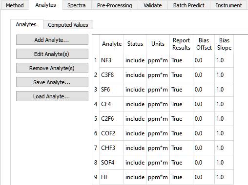
To edit an analyte, highlight its row in the analyte table, and then click 'Edit Analyte'. If you select multiple rows in the table, you can edit multiple analytes at a time. Here is the Dialog that allows editing an analyte:
Note that the Analyte Name cannot be edited; once an analyte is added to a method, its name cannot be changed. This is because the analyte name serves as a key for organizing Standards and Results.
Computed Values
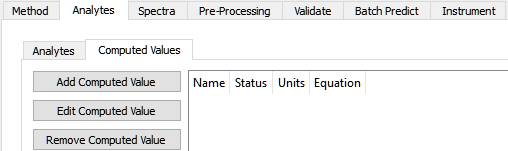
A computed value is calculated using Analyte results, using a supplied equation. It is sometimes used to calculate a percentage from a concentration, or to ratio two concentrations.
Clicking the 'Add Computed Value' button, this dialog is shown:
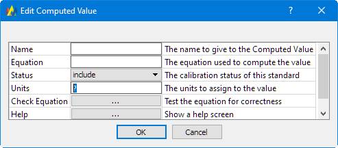
It's self-explanatory except for the 'Equation'. The 'Help' button displays this:
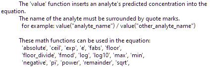
An example equation, given the analytes in this tutorial method, might be:
The Spectra Tab
The Spectra Tab has two sub-tabs: Standards and Inteferents.
A Standard is the spectrum of a pure Analyte. It is used to generate calibration information for predicting concentrations of unknowns. These pieces of information must be known about the Standard: its concentration, temperature, pressure and pathlength, often referred to using the intials 'C,T,P,L'.
An interferent is a spectrum which also has absorbance features in the same spectral region as the standard. Such spectra must be added to the standard as an interferent so that the interferent absorbances can be accounted for.
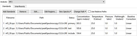
On the left is a list of Analytes. As a different analyte is selected, the Standards table changes to display the Standards for the selected Analyte. The Standards table has these columns: Filename, Path, Status, Concentration, Temperature, Pressure, and Pathlength, and Baseline Correction. The standards table can be sorted by clicking on any of the column headers. For instance, to sort the table by Concentration, click on the 'Concentration' column header.
| Filename | The filename containing this Standard's spectrum. |
| Path | The folder the file is in. |
| Status | This can be include, exclude, primary, or test |
| Concentration | The known concentration of the Analyte in this Standard |
| Temperature | The temperature when the spectrum was collected |
| Pressure | The pressure when the spectrum was collected |
| Pathlength | The pathlength when spectrum was collected. |
| Baseline Correction | This can be None, Offset, Linear, or Curve. |
'Curve' should be used with care, because baseline corrections are applied individually to analysis regions, not to the entire spectrum. If 'Curve' is used over a narrow peak region, the peak will be flattened out.
Each standard can have a different baseline correction method assigned to it. NOTE: be careful using 'Curve' baseline correction. The curve correction may fit a peak and remove it from the calibration.
The Buttons on the Spectra Tab.
 |
Add spectra to the table of Standards |
 |
Edit the selected Standard or Standards. The concentration can only be edited if a single Standard is selected. |
 |
Remove the selected Standard or Standards |
 |
Edit the Analytical Regions for a Standard. See the 'Editing Regions' section below. |
 |
Change the folder that the Standards are located in. |
 |
View the Standard Spectra. |
 |
Change the paths of all standards and interferents to be relative to the location of the method file. |
The Path can be changed independently of the Filename; you may have separate folders containing Standards that share the same filename, but may have been pre-processed differently, or have different spectral resolutions, or have been acquired from different instruments. This allows the method developer to experiment during the development phase by switching between sets of Standards.
'Use Relative Paths' is useful when distributing methods to other computers. On another computer, the method may be installed in a different folder location. If the paths are relative to the method location, the method will be able to find the files.
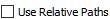
Standards can be edited by double-clicking on a row in the table, or selected one or more rows in the table and then clicking the 'Edit Standard(s)' button.
If editing a single standard, this dialog appears:
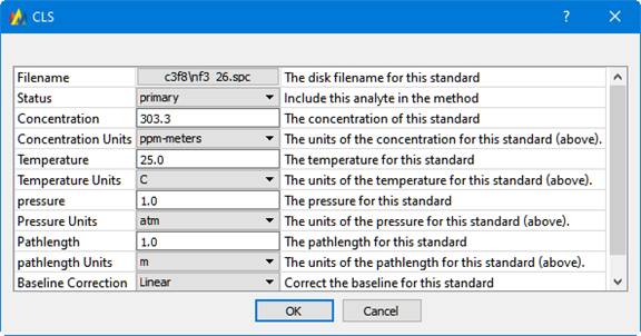
When editing multiple standards, this slightly different dialog appears, which contains a subset of the above fields, showing only those settings that would apply to multiple standards (Filename and Concentration are missing).
Note that this is another way to change the Path of multiple standards.
Note: when a method is loaded, if the standards cannot be found in the Path assigned to them, Peaks automatically looks in the method directory itself. This makes it easier to deploy methods to other computers.
Standard Status and Primary Status
A standard can be assigned a status of include, exclude, primary, or test. 'Include' and 'Primary' mean that the standard will be used in the CLS calibration for the Analyte. 'Exclude' means to ignore the standard. Ignore can be useful when developing a method, to see what result leaving the Standard out will have. 'Test' means the standard will be used in method validation, to see if the CLS prediction calculates a concentration that agrees with the known concentration of the test standard.
For a given analyte, there can only be one primary standard. The primary standard has these special properties:
-
The analytical regions of the primary standard are used for automatic interferent analysis (more on this in the Regions and Interferents sections, below).
-
The primary standard's spectrum is used as the interferent spectrum when automatic interferent analysis detects interference.
-
When the given analyte has multiple standards, the primary standard is used as an initial estimate to find the bracketing standards.
So, in the case where an analyte has multiple standards, care should be taken in selecting the primary standard, and also in selecting the analytical regions for the primary standard.
Editing Regions
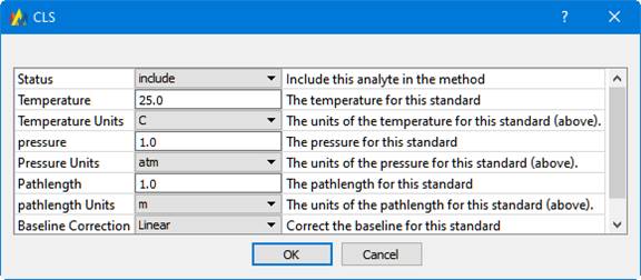
Analytes have spectral regions that contain information specific to that analyte. Clicking the 'Edit Regions' button brings up this dialog:
On this dialog, analytical regions are assigned to Standards. In this example the 'nf3_26.spc' spectrum is displayed.
Right-clicking the mouse on the spectral display will create two 'region markers', which are the vertical bars. The bars can be moved by dragging them with the left mouse button. The table below the spectral display tabulates the regions. An entry in the table can be edited directly by double-clicking on a cell in the table. In addition the 'Actions' button allows the region table to be saved, or for a saved table to be loaded.
The 'Apply this region to all the Calibration Standards for this Analyte' checkbox does exactly what it says. It will copy the regions to all the calibration standards for the currently selected Analyte. However, it is common to use a different set of regions for high versus low concentrations of an analyte.
Analytes usually have spectral regions that contain information specific to that analyte. Specifying spectral regions will improve the results and make the analysis faster.
The Interferents Tab
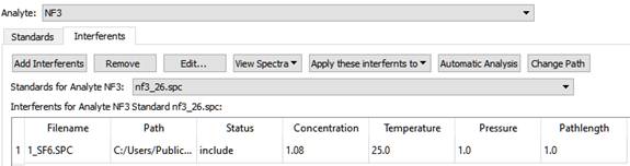
For a given Analyte and Standard pair, it is possible that other Analytes have significant absorbance in the given Analyte's analysis regions. These are called 'interferents', and they must be included in the calibration for the given analyte. This tab allows you to define interferents for the given analyte and standard.
An interferent does not have to be an Analyte or Standard in the method; you can include any spectrum. Just like Standards, the concentration, temperature, pressure and pathlength of the interferent spectra have to be known.
This can be a tedious operation, but there are some short cuts built into this software to make the job easier.
First of all, you can define the interferents for one Standard, and then apply them to all other standards for the given analyte, or to all standards for all analytes. Then you can edit the interferents for each Analyte and Standard by removing or excluding those interferents, which are not applicable to the analysis.
Automatic Interferent Analysis
Second, you can use the 'Automatic Analysis' function. This identifies interferences among the analytes and standards that are included in the method. Using the analysis regions defined for the primary standard for each analyte, it looks for overlap with the analysis regions of all the other primary standards. When any overlap is found, that other primary standard is added to the interferents of all the standards for the given analyte.
The Validation Tab
Validation means testing the CLS method against known data. You must have assigned some Standards to the 'Test' set in order to validate the selected Analyte.
The buttons at the top of the tab:

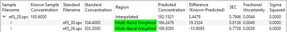
Choose the Analyte to validate from the drop-list of Analytes, and click the 'Validate' button. The table will be filled with results. The 'NF3' analyte was used for this discussion.

The final result is displayed. Clicking on the '>' icon next to the 'Sample Filename' will reveal more detail:
And clicking again on the newly revealed '>' icons will show more detail:
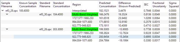
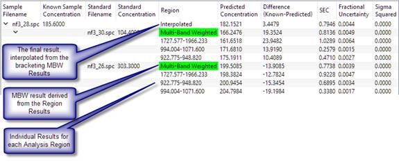
From the bottom up, a concentration is calculated for each analysis region for each standard. The individual analysis region results are combined using 'multi-band weighting' (see Reference 1). The MBW results that bracket the unknown are found, and the final result is interpolated from the two bracketing MBW results.
Bracketing means to find the standard with the best prediction that is above that standard's known concentration, and the best prediction that is below another standard's known concentration. The concentration of the unknown will lie somewhere between the two brackets. The two standards used in the interpolation are called the 'bracketing standards'. In the simple example above, there are only two standards, which conveniently bracket the test spectrum. In more complex methods, the software may have to choose between multiple standards to select the two that bracket the unknown.
For a given standard, the absolute value of the predicted concentration minus the standard concentration, divided by the standard concentration, gives a relative 'closeness' value. It measures how close the concentration predicted using that standard is to the standard's known concentration. For the low side, only those standards with a predicted concentration greater than the standard's known concentration are considered, and the standard with the lowest relative closeness value is chosen. On the high side, only those standards with a predicted result less than the standard's know concentration are considered.
Now consider a more complicated case. For the Analyte C3F8, the Standards table can be configured like this:
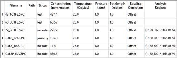
There are two test spectra, both of which are bracketed by the calibration standards. The results are:
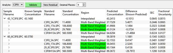
The bracketing standards used for the final interpolated result are highlighted in green.
Once the two bracketing standards are selected, the final value is interpolated using a weighting based on the relative closeness values used in finding the brackets.
Residuals and Statistics
The residual is what remains after the contributions of the analytes and any interferents are removed from the sample spectrum.
The residual for each result for any row in the results table can be viewed by highlighting that row and then clicking the 'View Residual' button. A smaller residual indicates a better result.
The spectral residual is used to calculate statistics that indicate how well the model is performing for a given prediction. SEC is the 'Standard Error of Concentration', see Reference 1. Fractional Uncertainty, also known as UCR, is SEC / (Predicted Concentration). Sigma Squared, or S2, is the estimated variance in the residual.
Notice how the predicted concentration for the high concentration test sample, C3F8H13A.SPC, the last one in the table, is way off from the known. This is because of non-linearity in the data: absorbance versus concentration is not a straight line, especially at higher concentrations. This is why a good method should include standards at many representative concentration values, and why interpolation between brackets is needed.
The Batch Predict Tab
This tool allows you to predict the concentrations of analytes in unknown samples.
There are two sub-tabs: Files and Results. Use the 'Add Files' button to add files to the list, and then click the 'Predict' button to generate the predictions, which will be displayed on the 'Results' tab.
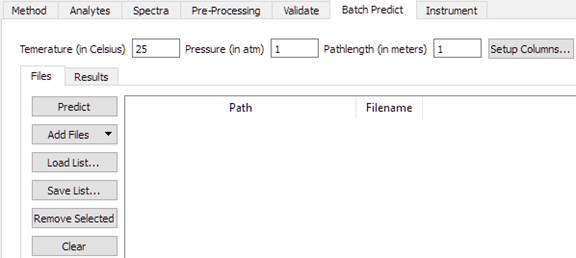
To analyze samples, the temperature, pressure, and pathlength of the samples must be known. These may be set using the edit fields on this tool. If you get unexpected results, the most likely cause is incorrect settings for these parameters.
The 'Setup Columns' button will display this dialog:
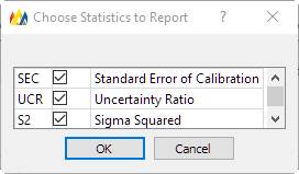
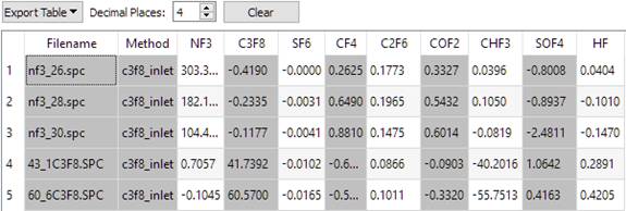
For the purposes of this tutorial, all the Check Boxes were un-checked, only the predicted concentration of each analyte is displayed.
To generate the results shown below, on the 'Spectra' tab, 'All Standards for All Analytes' was used on the 'View Spectra' button menu to load all the spectra into a window. Then, back on the 'Batch Predict / Files' screen, 'All Visible Files in Window' was selected from the 'Add Files' button menu.
References
-
D.M. Haaland and R.G. Easterling, 'Improved Sensitivity of Infrared Spectroscopy by the Application of Least Squares Methods,' Appl. Spectrosc. 34(5):539-548 (1980).
-
D.M. Haaland and R.G. Easterling, 'Application of New Least-Squares Methods for the Quantitative Infrared Analysis of Multicomponent Samples,' Appl. Spectrosc. 36(6):665-673 (1982).
-
D.M. Haaland, R.G. Easterling and D.A. Vopicka, 'Multivariate Least-Squares Methods Applied to the Quantitative Spectral Analysis of Multicomponent Samples,' Appl. Spectrosc. 39(1):73-84 (1985).
-
W.C. Hamilton, Statistics in Physical Science, Ronald Press Co., New York, 1964, Chapter 4.
-
Richard Kramer, Chemometric Techniques for Quantitative Analysis, Marcel Dekker Inc., New York, 1998, Chapter 3.