Peak Fitting (aka Curve Fitting) in Peak® Spectroscopy Software
Overview
Peak Fitting uses the Levenberg-Marquardt (LMFit) algorithm, which is widely used for non-linear curve-fitting problems. LMFit is well documented in the literature. From starting estimates it varies peak parameters, calculates a spectrum from those peaks, and evaluates the goodness of fit to the sample spectrum. The metric used to calculate goodness of fit is X2 (Chi-squared), which is the sum of the squared residual spectrum. The residual is the sample spectrum minus the calculated spectrum. LMFit is iterative and requires initial user input. The resulting fit is only as good as the initial peak estimates that are provided. LMFit will always find a solution, but that doesn't mean the solution is optimal or even valid. There can be a number of answers to a non-linear problem. Some solutions may be local minima but are not actually the best fit. This is especially likely if the initial peak estimates are far from the real answer. Another problem is over-fitting. Any spectrum can be fitted provided enough starting peaks, but those peaks may not have a corresponding real peak in the sample. The user is responsible for providing good input and for interpreting the results.
General Guidelines
- Peak Fitting works best on small spectral regions containing the overlapping peaks.
- Before launching the Peak Fitting application, zoom in on the spectral region you want to fit. The displayed region will be used for the peak fitting.
- If the data is noisy, results may benefit from smoothing before peak fitting.
- If the data has a sloping baseline, the results may benefit from baseline correction before peak fitting.
- It is important to account for all peaks, including 'buried' peaks.
Tutorial
This tutorial is an example of using peak fitting for protein secondary-structure analysis. The broad amide I band (~1700-1600 cm-1) is decomposed into several Gaussian/Lorentzian sub-bands that correspond to alpha-helix, beta-sheet, beta-turn and random-coil motifs. The fitted areas are converted into % secondary structure.
- Load the 'synthetic_protein.spc' datafile into a workspace. It is installed in the 'peakFit' sub-folder under the PeakSpectroscpy Documents folder.
- In the 'Analysis' toolbox, choose 'Peak Fitting'.
- Click the 'Load Peak Fitting Application' button.
- Click the 'Load Estimates Table' button and select the file 'synthetic protein.pfit'
The 'synthetic_protein.spc' was calculated using the table below. The peak shapes are all Lorentzian. These peaks are a simulation of a Mid-Infrared Protein Absorbance. Also in the peakFit sub-folder is a saved Peak Estimates table, named 'synthetic_protein.pfit'.
| Center | Amplitude | FWHH |
| 1627.9 | 1.00 | 9.5 |
| 1636.7 | 0.10 | 9.75 |
| 1645.7 | 0.25 | 10.2 |
| 1656.3 | 0.65 | 10.25 |
| 1666.7 | 0.36 | 9.35 |
| 1678.2 | 0.13 | 10.05 |
| 1690.8 | 0.05 | 9.75 |
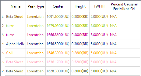
The Peak Estimates Table
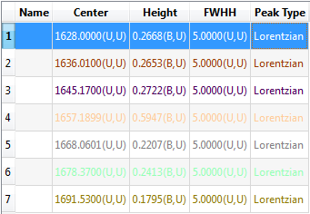
The Estimate Table looks like this. The designations such as (UU) after the Center, Height and FWHH encode constraints on those settings. A 'B' after a value in the table denotes that the Bounds Handling for that value is Bounded. If the mode were Fixed it would have 'F' and if it were Unbounded it will be 'U'. For instance, '(B,U') after the Height values means that the Low Bound is Bounded and the High Bound is Unbounded. Constraints can be applied using the 'Edit Peak' button.
 |
| synthetic_protein.pfit |
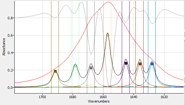
After loading the spectrum and the estimates table, the click the 'Fit Peaks' button. The fitting will be performed and the results displayed:
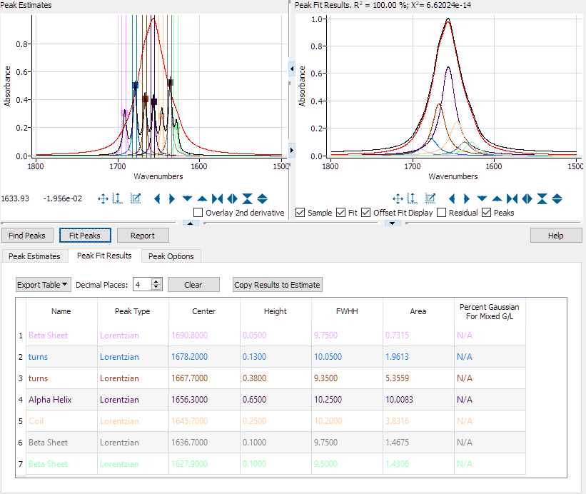 |
| Peak Fit Results. |
Manual Peak Selection
The first step in Peak Fitting is to tell the program the nominal positions of the peaks that comprise the spectrum. This can be done manually using the mouse, or by clicking the 'Add Peak' button, or by clicking the 'Find Peaks' button or by loading a saved Peak Estimates table.
Peak Selection with the Mouse
It helps to overlay the 2nd derivative by checking the '2nd derivative' box. The 2nd derivative is useful for finding buried peaks. A minimum in the 2nd derivative is the location of a peak.
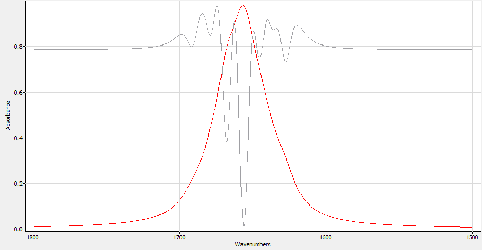 |
| Spectrum with overlaid 2nd Derivative |
To manually create a peak, right-click the mouse at a peak location. A peak marker is created is created at the mouse location. The peak marker consists of three elements: the Center marker and two width markers. The width initially is set to the default width provided in the Peak Options table.
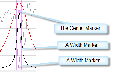 |
| A Peak Marker. |
The position, height, and width of the peak can be changed by dragging a marker with the left mouse button. When positioned over the Center Marker, the mouse cursor changes to indicate that the peak can be moved up and down and left and right. Moving the Center Marker moves the Width Markers along with it.
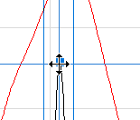 |
| The Peak Center Marker. |
When positioned over a vertical width marker, the mouse cursor changes to indicate that the width marker can be moved. Moving a width marker automatically moves the other width marker as well but leaves the Center Marker where it is.
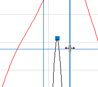 |
| The Peak Width Markers. |
When a peak marker is created with the mouse, an entry in the 'Peak Estimates' table is made corresponding to that peak. To remove a peak marker using the mouse, position the mouse over either the center marker or one of the width markers, and right-click. Also, the row corresponding to the peak in the Peak Estimates table can be selected and then the 'Remove Peak' button clicked. The left mouse button can still be used to expand (zoom in) on the spectral display, as long as it is not on a marker when the left mouse button is pressed.
Adding Peaks with the Keyboard
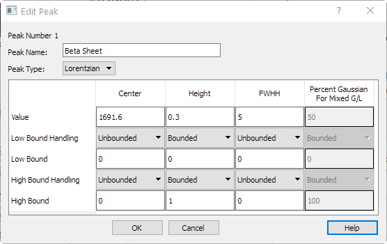 |
| Editing a Peak. |
The peak Center, Height, and FWHH can be entered manually. In addition, a peak can be given a name. A name can be useful in the analysis of the peaks. For instance, in this synthetic protein spectrum, peaks can be assigned to Beta Sheets, Alpha Sheets, Amide bands, and so forth. The 'Bound Handling' entries allow for restricting the peak search. The choices are:
| Unbounded | Allow the 'Value' to vary without any restrictions. |
| Bounded | Restrict the 'Value' to be in the range of 'Low Bound' and/or 'High Bound'. |
| Fixed | Do not allow the 'Value' to change during the peak fitting optimization. |
The 'Low Bound' value is only applied when 'Low Bound Handling' is set to 'Bounded' and the 'High Bound' value is only applied when 'High Bound Handling' is set to 'Bounded'. Note: there is nothing to restrict a peak height from becoming negative during LMFit. So, by default the Height Low Bound is set to 0, and the Height Low Bound Handling is set to Bounded.
Automatic Peak Selection
Clicking the 'Find Peaks' button will perform a 2nd derivative analysis of the spectrum and select peaks on that basis. 'Find Peaks' can be useful, but manually selecting peaks usually yields better results because the eye of an analyst is better at discerning fine structure than a computer algorithm. In this graphic, the 2nd derivative overlay was used to select the positions of the peaks:
 |
| Automatic Peak Finding. |
And the table of Peak Estimates looks like this:
 |
| Automatic Peak Finding. |
Automating (Batch Processing) Peak Fitting
The batch processing that is built into Peak can be used to automate peak fitting. This allows un-attended analysis of samples, and the ability to analyze many samples at once. To set this up,
- First, create a peak estimate table as described above and save a .pfit peak fitting model.
- Click on 'Batch Processor' in the 'Advanced' toolbox.
- Click on 'Create a new Sequence'
- Click on the 'Analysis' tab.
- Higlight 'Peak Fitting' and click the 'Add to Sequence' button. The peak fitting options table appears.
- Load a peak estimate table .pfit file.
- To save the calculated peaks as individual .csv files, click the 'Save Peaks' checkbox, and choose a folder as the destination for the these files. The files will be saved in a sub-folder (named after the sample filename) of the destination folder. The table of results is also saved.
- Save save the batch processing sequence.
If smoothing or baseline correction need to be done prior to the peak fitting, these manipulations can be added to the sequence.